前两篇文章我们讨论了逻辑回归的基本概念与决策边界的概念,并且具体进行了编码实现。本文我们使用sklearn为我们提供的逻辑回归类来实现逻辑回归,并且讨论有关正则化的问题。
一、逻辑回归的模型正则化
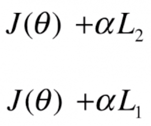
在机器学习算法笔记(二十二):L1正则、L2正则与弹性网中,我们介绍了两种正则化的方法,分别是 L1 正则和 L2 正则:
然而在本文中,我们来看一个对于正则化新的表示方式,但其实原理是和之前完全一样的:
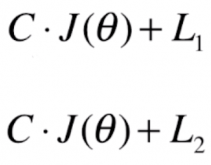
这么做其实就是在 J(θ) 之前加入了一个超参数 C。使用这种方式与一开始的形式唯一的区别就是我们“不得不”进行正则化(因为 L1 和 L2 的系数不可能为零),只能调整正则化项和损失函数之间的权重。正因如此,在逻辑回归中对模型进行正则化时更偏向这种形式,sklearn中对逻辑回归的实现就是这种方式。
二、使用sklearn实现逻辑回归并引入正则化
新建一个工程,创建一个main.py文件,实现以下代码:
import numpy as np
import matplotlib.pyplot as plt

#生成测试数据
np.random.seed(666)
X = np.random.normal(0, 1, size=(200, 2))
y = np.array((X[:,0]**2+X[:,1])<1.5, dtype='int')
for _ in range(20):
    y[np.random.randint(200)] = 1

#绘制决策边界
def plot_decision_boundary(model, axis):
    x0, x1 = np.meshgrid(
        np.linspace(axis[0], axis[1], int((axis[1] - axis[0]) * 100)).reshape(-1, 1),
        np.linspace(axis[2], axis[3], int((axis[3] - axis[2]) * 100)).reshape(-1, 1),
    )
    X_new = np.c_[x0.ravel(), x1.ravel()]

    y_predict = model.predict(X_new)
    zz = y_predict.reshape(x0.shape)

    from matplotlib.colors import ListedColormap
    custom_cmap = ListedColormap(['#EF9A9A', '#FFF59D', '#90CAF9'])

    plt.contourf(x0, x1, zz, linewidth=5, cmap=custom_cmap)

from sklearn.model_selection import train_test_split

X_train, X_test, y_train, y_test = train_test_split(X, y, random_state=666)

from sklearn.preprocessing import PolynomialFeatures
from sklearn.pipeline import Pipeline
from sklearn.preprocessing import StandardScaler
from sklearn.linear_model import LogisticRegression

def PolynomialLogisticRegression(degree, C, penalty='l2'):
    """
    :param degree: 引入特征的阶数,默认为2
    :param C: 正则化式子中损失函数前的系数C,默认为1
    :param penalty: 使用L1正则还是L2正则,默认L2
    """
    return Pipeline([
        ('poly', PolynomialFeatures(degree=degree)),
        ('std_scaler', StandardScaler()),
        ('log_reg', LogisticRegression(C=C, penalty=penalty))
    ])

poly_log_reg = PolynomialLogisticRegression(degree=2, C=1, penalty="l2")
poly_log_reg.fit(X_train, y_train)
print(poly_log_reg.score(X_train, y_train)) #prints: 0.9133333333333333
print(poly_log_reg.score(X_test, y_test)) #prints: 0.94

plot_decision_boundary(poly_log_reg, axis=[-4, 4, -4, 4])
plt.scatter(X[y==0,0], X[y==0,1])
plt.scatter(X[y==1,0], X[y==1,1])
plt.show()
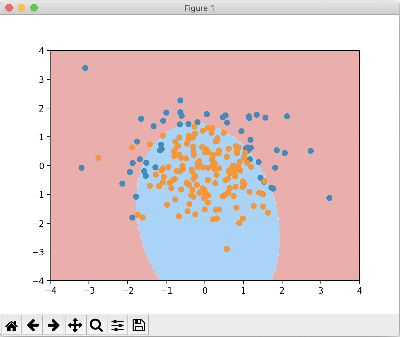
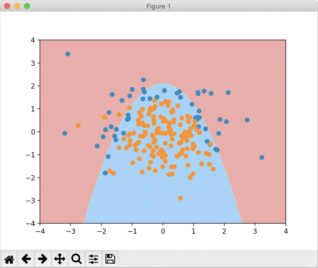
绘制出来的图像如下:
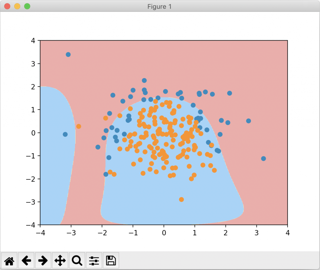
下面我们把degree设成20,也就是过拟合的情况,看看这个时候绘制的图像:
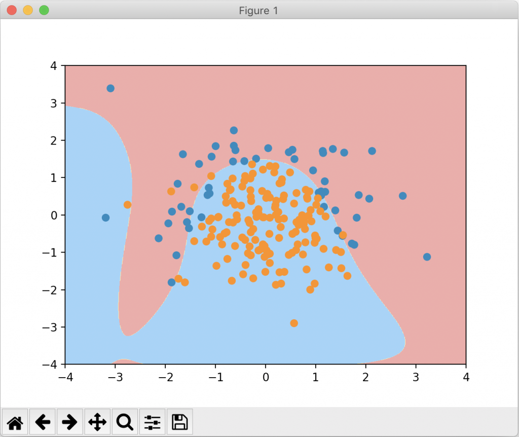
我们可以看到绘制的决策边界弯弯曲曲,这是典型的过拟合的表现。接下来我们把 C 设成 0.1,一个较小的值,再来看一下绘制的图像:
可以看到这个形状虽然比较奇怪,但是相比于C=1时已经没有那么的弯弯曲曲,更倾向于degree=2的情况。下面我们换用L1正则项来看一看:
由于数据集相对较简单,过拟合不够明显,正则化后的准确度反而降低了。但若我们通过决策边界来看,使用 L1 正则项的效果显然最接近原来degree=2的图像。
使用 L1正则项能使一些次数较大的多项式项前面的系数为零(这在第二十一篇笔记中讨论过),使得整个决策边界不会弯弯曲曲,很好的纠正了过拟合的结果。
在面对实际数据时,我们是不知道degree是多少、C是多少、正则项使用 L1 或者 L2 才是最合适的,这些都属于超参数,我们需要使用网格搜索来找出对应的最佳参数应用到算法中。